Unlock the Power of the Laplace Transform: A Visual Guide
The Laplace transform is a powerful mathematical tool, especially for solving differential equations. While it’s straightforward to learn the mechanics of using it, understanding what it actually *does* can be elusive.
This guide aims to demystify the Laplace transform by visualizing its inner workings, much like understanding an internal combustion engine rather than just driving a car. We’ll build a conceptual understanding of this transform, explore its definition, and see how it simplifies complex problems.
What You’ll Learn:
- The fundamental concepts behind the Laplace transform, including the role of exponential functions and the s-plane.
- A visual and intuitive explanation of the Laplace transform’s definition and how it reveals the exponential components of a function.
- How the Laplace transform converts differential equations into algebraic problems.
- An introduction to the concept of ‘poles’ and their significance in understanding transformed functions.
- A practical example of using the Laplace transform to analyze a function like cosine.
Prerequisites:
- Basic understanding of exponential functions (e^x).
- Familiarity with complex numbers (including imaginary parts).
- A foundational grasp of calculus, particularly integration.
The Problem: Decomposing Functions into Exponentials
Before diving into the Laplace transform itself, it’s crucial to understand the problem it aims to solve. Many functions, particularly those encountered in physics and engineering, can be represented as combinations of exponential functions. The Laplace transform acts as a mathematical machine that can take a function and reveal these underlying exponential components.
1. Understanding Exponential Functions and the s-Plane
The core of the Laplace transform lies in understanding exponential functions of the form e^(st), where ‘t’ represents time and ‘s’ is a complex number. The value of ‘s’ dictates the behavior of the exponential function:
- If ‘s’ has an imaginary part, the function’s output rotates in the complex plane as time progresses.
- If the real part of ‘s’ is negative, the function’s magnitude decays towards zero over time.
- If the real part of ‘s’ is positive, the function’s magnitude grows exponentially.
Engineers often refer to the complex plane of possible ‘s’ values as the s-plane. Each point on this plane can be thought of as representing a unique exponential function e^(st). The graphs of these functions visually represent their behavior: larger imaginary parts lead to faster oscillations, while the real part indicates decay or growth.
2. Functions as Combinations of Exponentials
A key insight is that many common functions can be expressed as sums of simpler exponential pieces. For example, the cosine function, cos(t), can be represented as the sum of two complex exponentials: 0.5 * e^(it) + 0.5 * e^(-it). More complex systems, like a driven harmonic oscillator, can be broken down into even more exponential components.
The goal of the Laplace transform is to provide a tool that can ‘pump in’ a function (or a differential equation describing it) and reveal the specific exponential pieces it comprises – essentially identifying the values of ‘s’ and their corresponding coefficients.
3. The Derivative Simplification
A significant advantage of using exponential functions is how their derivatives behave. The derivative of e^(st) with respect to ‘t’ is simply s * e^(st).
This means that differentiation in the time domain becomes simple multiplication in the ‘s’ domain. This property is what allows the Laplace transform to convert differential equations into algebraic equations, making them much easier to solve.
The Laplace Transform: Definition and Visualization
The Laplace transform is a type of ‘transform’ operation that takes an entire function as input and produces a new function as output. If the original function is denoted by f(t) (where ‘t’ is time), its Laplace transform is typically denoted by F(s) (where ‘s’ is a complex number).
4. The Formal Definition
The Laplace transform of a function f(t) is defined by the integral:
F(s) = ∫[0 to ∞] f(t) * e^(-st) dt
This definition involves two main steps:
- Multiply the original function
f(t)bye^(-st). - Integrate the result with respect to time ‘t’ from 0 to infinity.
The parameter ‘s’ is a complex number that acts as the input to the new transformed function F(s). By varying ‘s’ across the s-plane, the transform essentially ‘sniffs out’ which exponential functions e^(st) are present in the original function f(t).
5. Understanding the Integral: Area and Averages
Interpreting the integral ∫[0 to ∞] e^(-st) dt provides crucial intuition. For a real value of ‘s’, this integral represents the area under the graph of e^(-st) from 0 to infinity.
If s=1, the area is 1. As ‘s’ decreases towards 0, the area increases towards infinity.
A more general way to visualize the integral, especially for complex ‘s’, is to think of it as summing up the ‘average values’ of the function over successive unit intervals of time. Imagine a pool of water representing the function’s values over an interval; its height is the average value. As we sum these averages (represented as vectors) across all time intervals from 0 to infinity, the final point of this spiraling sum represents the value of the integral.
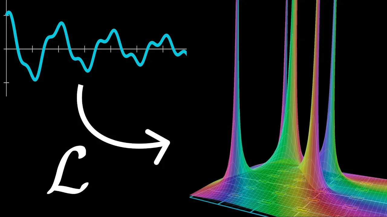
6. Poles: Detecting Exponential Components
A key concept revealed by the Laplace transform is the idea of poles. When the Laplace transform F(s) is plotted over the s-plane, sharp spikes (poles) appear at values of ‘s’ that correspond to the exponential components of the original function f(t).
For example, the Laplace transform of the constant function f(t) = 1 is F(s) = 1/s. This function has a pole at s=0, indicating the presence of an exponential component related to e^(0*t) = 1.
More generally, the Laplace transform of an exponential function e^(at) is 1/(s-a). This function has a pole at s=a. This is a fundamental relationship: poles in the transformed function F(s) reveal the exponents ‘a’ of the exponential pieces e^(at) in the original function f(t).
7. Linearity and Combinations
The Laplace transform is a linear operation. This means that if a function is a sum of other functions, its Laplace transform is the sum of their individual Laplace transforms. For instance, if f(t) = c1*f1(t) + c2*f2(t), then F(s) = c1*F1(s) + c2*F2(s).
Using this property and the fact that the transform of e^(at) is 1/(s-a), we can find the transform of functions like cosine. Since cos(t) = 0.5*e^(it) + 0.5*e^(-it), its Laplace transform is:
F(s) = 0.5 * (1/(s-i)) + 0.5 * (1/(s+i))
This resulting function will have poles at s=i and s=-i, directly corresponding to the exponential components of the cosine function.
Analytic Continuation: Extending the Domain
A nuanced aspect of the Laplace transform is that the integral defining it often only converges for a specific region of the s-plane (e.g., where the real part of ‘s’ is positive). However, the resulting function (like 1/s or 1/(s-a)) can often be extended to a larger domain, even where the original integral doesn’t converge. This process is called analytic continuation.
Complex-valued functions are highly constrained: if a function is well-behaved (has a derivative), its analytic continuation is unique. This allows us to understand the full behavior of the transformed function, including its poles, even in regions where the direct integration doesn’t make sense. The plots often shown for Laplace transforms represent this analytic continuation, revealing all the poles that characterize the original function’s exponential makeup.
Conclusion
The Laplace transform is more than just a computational tool; it’s a lens through which we can view functions and differential equations. By transforming a problem from the time domain to the s-plane, we can simplify complex operations like differentiation into algebraic manipulations and expose the fundamental exponential building blocks of functions through the location of poles. Understanding these underlying principles not only makes the process of solving equations more intuitive but also reveals the elegance of the mathematical machinery at play.
Source: But what is a Laplace Transform? (YouTube)