Understand Phase Transitions With a Liquid-Vapor Simulation

Simulating and Understanding Phase Transitions in a Liquid-Vapor Model

Phase transitions, such as ice melting into water or water boiling into steam, are fundamental phenomena in physics and chemistry. While we intuitively understand these changes, the underlying principles can be complex. This article will guide you through understanding and simulating a simplified liquid-vapor model, which exhibits phase transitions. We will explore the concept of phase transitions, delve into the crucial Boltzmann formula, and learn how to build and interpret a simulation that visualizes these changes.

What is a Phase Transition?

A phase transition is not a chemical reaction; the molecules themselves remain the same. Instead, it represents a change in how these molecules interact and organize themselves. For example:

• Ice: Molecules are locked in a rigid structure with long-range interactions.
• Water: Molecules are less structured, with some long-range interactions allowing for wave propagation (ripples).
• Steam: Molecules are highly dispersed with minimal interaction between distant molecules.

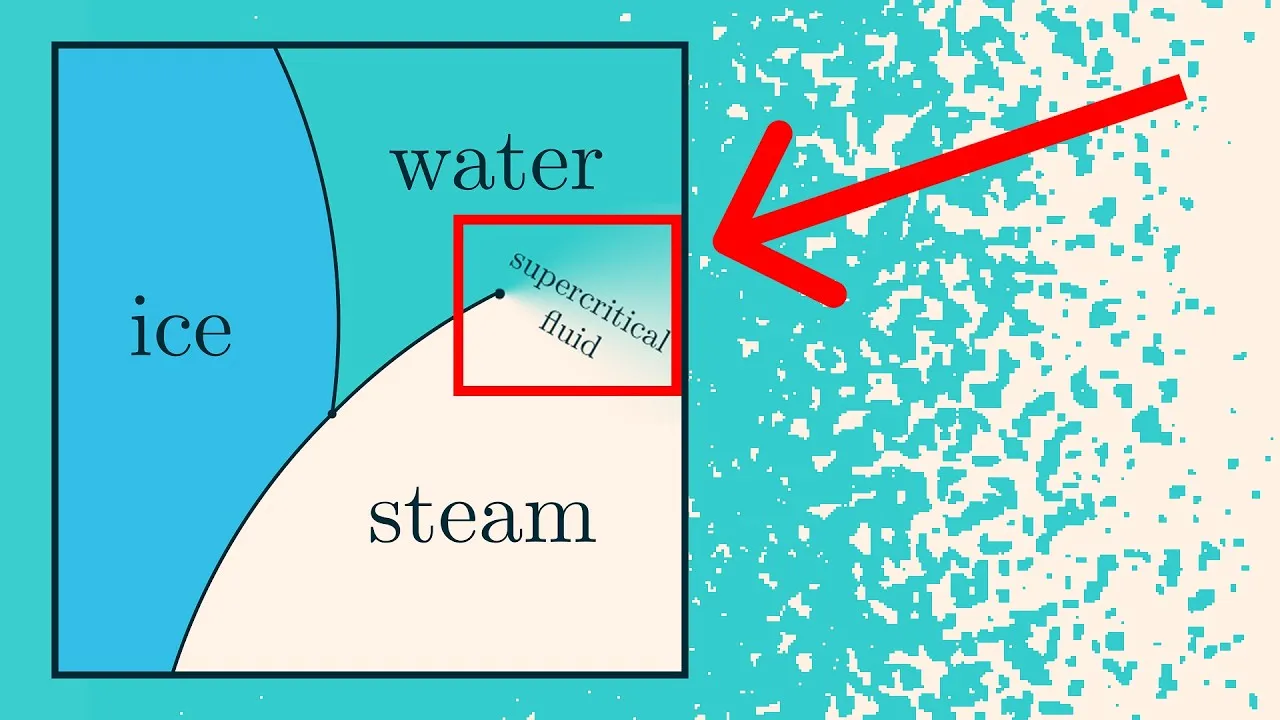
Phase diagrams, often seen in chemistry, illustrate the phases of matter (solid, liquid, gas) at different temperatures and pressures. Crossing the lines between these phases signifies a phase transition. It’s important to note that phase transitions describe the equilibrium behavior of a system after it has settled, not the dynamic process of change in real-time.

The Liquid-Vapor Simulation Model

We will be working with a discretized simulation where blue pixels represent molecules and white pixels represent empty space. The simulation’s behavior is controlled by two parameters:

• Temperature (T): Influences how important energy is. At high temperatures, molecular clumping matters less, and randomness dominates.
• Chemical Potential (μ): Acts as a proxy for pressure in this simulation. Higher chemical potential generally leads to more molecules on the screen, increasing density.

In this model:

• At high temperatures, varying the chemical potential leads to smooth changes in molecular density, similar to a supercritical fluid.
• At low temperatures, crossing a certain threshold triggers a phase transition. The density abruptly shifts from very low (gas-like) to very high (liquid-like), skipping intermediate values. In the simulation, this manifests as distinct regions of mostly blue or mostly white pixels, with sharp boundaries.

The Boltzmann Formula: The Heart of the Simulation

To understand how the simulation generates its probabilistic behavior, we need to introduce the Boltzmann formula. This formula describes the probability distribution of different microstates (specific configurations of all particles) in a system.

Why Use Randomness?

Simulating systems with a vast number of particles (like molecules in a teaspoon of water, ~10^23) using deterministic physics (Newton’s laws) is computationally impossible. Even with a few hundred particles, calculations become intractable. Instead, we use randomness as a powerful approximation.

The key idea is that for large systems, we are interested in the macrostate (overall behavior, like whether it’s liquid or gas) rather than the precise microstate of every single particle. Randomness serves as a proxy for our uncertainty about the exact microstate.

The Boltzmann Distribution

The probability (P) of observing a particular microstate (x) is proportional to the exponential of its energy (E) divided by the temperature (T):

P(x) ∝ exp(-E(x) / T)

(Note: Boltzmann’s constant ‘k’ is omitted by choosing appropriate units.)

Understanding Energy, Entropy, and Free Energy

The Boltzmann distribution implies:

• Higher energy states are less probable.
• The most likely energy level is determined by a balance between energy (E) and entropy (S, the number of microstates at a given energy).

This balance is captured by the free energy, defined as F = E – T*S. Nature seeks to minimize this free energy.

• At low temperatures, minimizing energy (E) is prioritized.
• At high temperatures, maximizing entropy (S) becomes more important.

This competition between energy and entropy, mediated by temperature, is the fundamental driver of phase transitions.

Building Your Own Simulation (Conceptual Steps)

The simulation samples microstates according to the Boltzmann distribution. Here’s a conceptual overview of how it works:

Step 1: Define the System and Energy

In our liquid-vapor model:

• The system is a grid of pixels.
• Molecules (blue pixels) prefer to be near each other but not too close (one molecule per pixel).
• Energy is defined as the negative of the number of adjacent molecule pairs. More adjacency means lower energy.

Step 2: Understand Temperature and Equilibrium

Temperature is defined as the quantity that equalizes when systems exchange energy. Mathematically, it’s related to the derivative of entropy with respect to energy (1/T = dS/dE). Intuitively, temperature governs how adding energy affects the number of available microstates.

Step 3: Deriving the Boltzmann Formula with a Heat Bath

By considering a small system in contact with a large heat bath (a system at a fixed temperature), and knowing that all microstates of the combined isolated system are equally likely, we can derive the Boltzmann distribution for the small system. The probability of a microstate depends on the number of compatible microstates in the heat bath, which, due to the heat bath’s size, is related to the exponential of its energy divided by the system’s temperature.

Step 4: Sampling Microstates (Kawasaki Dynamics)

Directly sampling from the Boltzmann distribution is inefficient due to the exponential number of microstates. Instead, simulations use algorithms like Kawasaki Dynamics (a type of Markov Chain Monte Carlo):

1. Select Pixels: Randomly choose two pixels.
2. Propose Swap: Consider swapping a molecule between these two pixels (if one has a molecule and the other doesn’t).
3. Calculate Energy Difference: Determine the change in energy (ΔE) if the swap occurs. This depends only on the local neighborhood of the chosen pixels.
4. Decide Probability: The probability of accepting the swap (and thus changing the microstate) is given by: P(accept) = min(1, exp(-ΔE / T)).
5. Repeat: Repeating this process over many steps gradually leads the system towards a state that accurately samples the Boltzmann distribution.

This method allows the simulation to evolve and eventually display the characteristic gas and liquid phases, and the transitions between them, as dictated by the temperature and chemical potential.

Key Takeaways

• Phase transitions arise from the competition between energy minimization and entropy maximization, governed by temperature.
• The Boltzmann formula provides the probability distribution for microstates in a system at a given temperature.
• Simulations use algorithms like Kawasaki Dynamics to efficiently sample these microstates and visualize phase transitions.

This simulation provides a visual and interactive way to grasp the fundamental concepts behind phase transitions, demonstrating how simple rules and probabilistic principles can lead to complex emergent behaviors in physical systems.

Source: Simulating and understanding phase change | Guest video by Vilas Winstein (YouTube)