Discover All Incomplete Cubes: A Mathematical Art Exploration

How to Discover All Incomplete Cubes: A Mathematical Art Exploration

This article delves into the mathematical underpinnings of Sol LeWitt’s artwork, “Variations of Incomplete Open Cubes.” You will learn how to approach a complex combinatorial problem by breaking it down, exploring its symmetries, and understanding the relationship between different configurations of incomplete cubes. We will investigate the concept of rotational equivalence and discover a method to count unique cube variations.

Understanding Sol LeWitt’s “Variations of Incomplete Open Cubes”

Sol LeWitt, a prominent figure in conceptual art, minimalism, and serial art, created “Variations of Incomplete Open Cubes.” This artwork presents a grid of small skeletal frames, each representing a unique way a cube can be incomplete. The art piece is a visual representation of a mathematical problem: enumerating all distinct incomplete open cubes under specific constraints.

What Defines an Incomplete Open Cube?

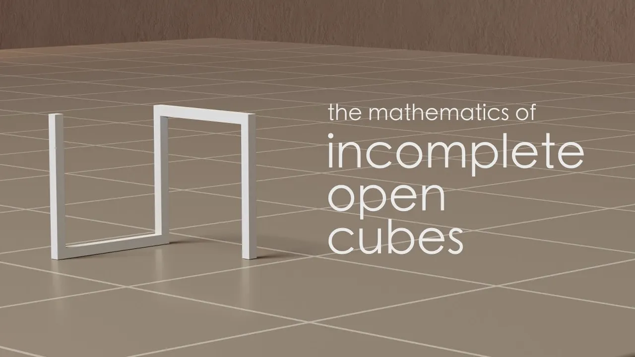
• Open Cube: A hollow cube framed by its 12 edges.
• Incomplete: Achieved by removing one or more edges from the open cube.
• Constraint 1 (Connectivity): The remaining edges must form a single connected component. The cube cannot fall apart into separate pieces.
• Constraint 2 (Dimensionality): The remaining edges must form a “properly three-dimensional” shape. This means it must have at least one edge along the height, width, and depth. Flat squares or single edges do not count.
• Constraint 3 (Rotational Equivalence): Different orientations of the same fundamental shape are considered identical. The artwork displays only one representative from each set of rotationally equivalent cubes.

LeWitt’s final artwork displays 122 rotationally unique incomplete open cubes. The challenge lies in understanding how to arrive at this number, which involves solving a non-trivial mathematical problem.

The Mathematical Problem: Counting Unique Cube Configurations

The core of this exploration is to understand the mathematical process behind LeWitt’s artwork. We will simplify the problem by initially focusing on rotational equivalence and relaxing the other constraints. This allows us to explore the fundamental symmetries of incomplete cubes.

Step 1: Understanding the Total Number of Possibilities

A cube has 12 edges. Each edge can either be present (‘on’) or absent (‘off’). This gives us two choices for each of the 12 edges. Using the principle of binary choices, the total number of possible configurations for incomplete open cubes is 2 raised to the power of the number of edges.

Calculation: 2¹² = 4096

This means there are 4096 potential incomplete open cubes before we consider any constraints or equivalences.

Step 2: Exploring Rotational Equivalence with a Simpler Case (Squares)

To grasp the complexity of rotational equivalence, we first consider the two-dimensional case: incomplete open squares. A square has 4 edges, so there are 2⁴ = 16 possible configurations.

By manually examining these 16 configurations, we can group them into families of shapes that are rotationally equivalent. For example:

• A single edge (e.g., the top edge) can be rotated into 4 positions, forming a family of 4.
• Two adjacent edges (e.g., top and left) can be rotated into 4 positions, forming a family of 4.
• Two parallel edges (e.g., top and bottom) can be rotated into 2 positions, forming a family of 2.
• A complete square is only equivalent to itself, forming a family of 1.
• An empty square (no edges) is also only equivalent to itself, forming a family of 1.

Summing the sizes of these families (4+4+2+4+1+1) gives us 16 total configurations. The number of unique families for squares is 6.

Step 3: Visualizing the Challenge in 3D

Extending this to cubes, a brute-force approach of manually sorting 4096 configurations and their rotations is extremely time-consuming and impractical. This is the challenge LeWitt faced.

Step 4: LeWitt’s Strategy: Divide and Conquer

LeWitt simplified the problem by breaking it down:

• Focusing on the Number of Edges: He realized that cubes with different numbers of edges could never be rotationally equivalent. He dedicated different pages of his notebooks to cubes with 3 edges, 4 edges, 5 edges, and so on.
• Organizing by Edge Count: The final artwork is arranged in rows, with each row representing cubes having a specific number of edges (e.g., the bottom row for 3-edge cubes).

Step 5: Developing a Mathematical Approach: Family Size and Symmetry

To find a formulaic solution, we need to understand the size of each rotational family. The key insight is the relationship between a cube’s symmetry and its family size.

• Symmetry and Lookalikes: A shape is symmetrical if it looks the same from multiple viewpoints. We can quantify this by identifying “lookalikes” – transformations that leave a cube appearing unchanged.
• The Core Relationship: The number of distinct orientations (family size) multiplied by the number of “lookalikes” for a given cube always equals 24 (the total number of rotational symmetries of a cube).

Formula: Family Size = 24 / Number of Lookalikes

Example:

• A cube with a single edge removed: It has 2 lookalikes (doing nothing, or rotating around the axis of that edge). Therefore, its family size is 24 / 2 = 12. This makes sense, as there are 12 distinct edges to remove.
• A complete cube: It has 24 lookalikes (it looks the same from every orientation). Its family size is 24 / 24 = 1.

Step 6: The Power of Notation: Edge Numbering and Complementary Pairs

LeWitt found that numbering the edges of the cube was more effective than labeling corners. This notation system revealed a crucial concept: complementary pairs.

• Complementary Pairs: If a cube is defined by the set of edges it *has*, its complement is defined by the set of edges it *lacks*. The total number of edges is 12.
• Exploiting Duality: If a cube has ‘n’ edges, its complement has ’12-n’ edges. This means a 4-edge cube is paired with an 8-edge cube, a 5-edge cube with a 7-edge cube, and so on.

By considering these complementary pairs, LeWitt could effectively cut his search effort in half, as solving for one automatically provided information about the other.

Step 7: Defining Transformations and Family Portraits

To systematically generate all members of a family, we need to define the possible transformations (rotations) of a cube. There are 24 such rotations, categorized by axes:

• Face Axes: Rotations around axes passing through the centers of opposite faces (9 rotations).
• Corner Axes: Rotations around axes passing through opposite vertices (8 rotations).
• Edge Axes: Rotations around axes passing through the midpoints of opposite edges (6 rotations).
• Identity: The original orientation (1 transformation).

A “family portrait” is created by applying all 24 transformations to a single cube. If a cube belongs to a family of size ‘k’, its family portrait will contain ‘k’ unique cubes, repeated 24/k times.

Step 8: Connecting Lookalikes, Family Size, and Total Count

The relationship Family Size = 24 / Number of Lookalikes is the key. By identifying the number of lookalikes for each type of cube (based on its structure and symmetry), we can determine its family size. Summing the sizes of all unique families will give the total count of rotationally unique incomplete open cubes. While LeWitt’s notebooks show his painstaking empirical process, mathematicians can use group theory and symmetry principles to arrive at the final count more directly.

Conclusion

Sol LeWitt’s artwork is a fascinating intersection of art and mathematics. By exploring “Variations of Incomplete Open Cubes,” we gain insight into how artists can engage with complex mathematical problems. The process of breaking down the problem, using symmetry, developing notation, and understanding rotational equivalence provides a powerful framework for tackling combinatorial challenges, demonstrating that even seemingly simple geometric forms can hide profound mathematical depth.

Source: Exploration & Epiphany | Guest video by Paul Dancstep (YouTube)