Unlock the Power of Laplace Transforms for Dynamic Systems
Have you ever wondered how to analyze complex systems that change over time, like a mass on a spring being pushed by an external force? These systems often start with messy, unpredictable behavior before settling into a steady rhythm. Understanding this initial “startup” period and predicting the final pattern can be challenging. This article will guide you through using Laplace transforms, a powerful mathematical tool, to simplify and solve these dynamic problems. You’ll learn how Laplace transforms turn difficult calculus problems into simpler algebra, making it easier to understand system behavior, predict outcomes, and find exact solutions.
What You’ll Learn
This guide will show you how to apply Laplace transforms to solve differential equations that describe dynamic systems. Specifically, you will learn:
- How Laplace transforms represent functions in a new “s-plane” and what poles in this plane tell you about system behavior like oscillation and decay.
- The key property that allows Laplace transforms to convert derivatives into algebraic multiplication, simplifying differential equations.
- A step-by-step method to transform a differential equation into an algebraic equation, solve it in the s-domain, and understand the system’s dynamics from its transformed solution.
- How initial conditions are automatically handled by this method.
Prerequisites
To get the most out of this guide, it’s helpful to have a basic understanding of:
- Functions and basic calculus (derivatives).
- Complex numbers and the complex plane.
- Exponential functions (like e^at) and trigonometric functions (like cosine).
Understanding the Basics: The s-Plane and Poles
Laplace transforms work by changing a function of time (like how a spring moves) into a new function that uses a complex number called ‘s’. This new function is viewed on something called the ‘s-plane’, which is simply a map of all possible complex numbers ‘s’.
Think of each point on the s-plane as holding information about a specific type of function. If ‘s’ has a large imaginary part, the original function likely oscillates a lot. If the real part of ‘s’ is negative, the function tends to fade away over time. If the real part is positive, the function grows without limit. These special points on the s-plane that reveal information about the original function are called ‘poles’.
The Laplace transform is like a translator. It takes a function of time and expresses it in a new language using ‘s’. A key idea is that if your original function can be broken down into simple exponential pieces, then the transformed version will have poles at specific locations. Each pole tells you about an exponential piece hidden within the original function.
Key Properties of Laplace Transforms
There are two main properties that make Laplace transforms so useful:
- Exponential Transformation: An exponential function like e^at transforms into a simple fraction: 1/(s – a). This fraction has a pole at s = a, directly showing the ‘a’ from the original exponential.
- Linearity: If you have a combination of functions (like a sum or scaled version), its Laplace transform is the same as transforming each function separately and then combining the results. This means if your original function is made of several exponential parts, the transformed function will be a sum of fractions, each with its own pole.
These properties allow us to understand the behavior of a system just by looking at the poles in its transformed function. Poles with negative real parts suggest stability and decay, while poles with positive real parts indicate instability and growth.
Turning Calculus into Algebra: The Derivative Property
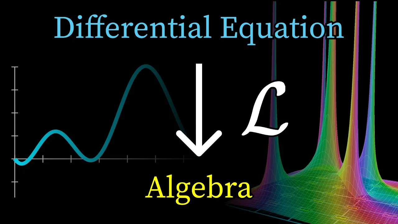
One of the most powerful aspects of Laplace transforms is how they handle derivatives. When you take the derivative of a function with respect to time, its Laplace transform turns this calculus operation into a simple algebraic multiplication.
Specifically, the Laplace transform of the derivative of a function, let’s call it f(t), is equal to ‘s’ multiplied by the Laplace transform of f(t), minus the initial value of f(t) at time zero (f(0)).
The Rule: Transform(f'(t)) = s * Transform(f(t)) – f(0)
This might seem small, but it’s huge! It means that complicated differential equations, which involve derivatives, can be converted into algebraic equations involving ‘s’. Algebra is much easier to work with than calculus.
Why it’s Important: This property is the key to solving differential equations. It also automatically includes the initial conditions (like the starting position or velocity) of the system, which are crucial for finding the correct specific solution.
Step-by-Step: Solving a Differential Equation
Let’s see how this works with an example: a mass on a spring with an added external force. The motion of such a system is described by a differential equation. Our goal is to find the function that describes the mass’s position over time.
Step 1: Write Down the Differential Equation
Imagine a mass (m) on a spring (with spring constant k) that also has some friction (damping coefficient, mu). On top of that, an external force (like wind) pushes it. The equation might look something like this:
m * x”(t) + mu * x'(t) + k * x(t) = F(t)
Here, x(t) is the position, x'(t) is the velocity, and x”(t) is the acceleration. F(t) is the external force.
Step 2: Take the Laplace Transform of Both Sides
Apply the Laplace transform to every term in the equation. We’ll use X(s) to represent the Laplace transform of x(t).
- The transform of x(t) is X(s).
- The transform of x'(t) is s*X(s) – x(0) (where x(0) is the initial position).
- The transform of x”(t) is s²*X(s) – s*x(0) – x'(0) (where x'(0) is the initial velocity).
The transform of the external force, F(t), will depend on what F(t) is (e.g., a cosine function). Let’s say the transform of F(t) is F(s).
So, the equation becomes:
m * [s²*X(s) – s*x(0) – x'(0)] + mu * [s*X(s) – x(0)] + k * X(s) = F(s)
Step 3: Simplify and Solve for X(s)
Now, rearrange the equation to get all terms with X(s) on one side and everything else on the other.
First, let’s assume the initial position x(0) and initial velocity x'(0) are both zero to make it simpler. This means the system starts at rest.
m*s²*X(s) + mu*s*X(s) + k*X(s) = F(s)
Factor out X(s):
X(s) * [m*s² + mu*s + k] = F(s)
Now, isolate X(s):
X(s) = F(s) / (m*s² + mu*s + k)
This expression for X(s) is the Laplace transform of the solution. It contains all the information about how the system will behave.
Step 4: Analyze the Transformed Solution (X(s))
Even without finding the exact time-based solution yet, we can learn a lot by looking at X(s). The key is to find the ‘poles’ – the values of ‘s’ that make the denominator zero.
- Poles from the Denominator (m*s² + mu*s + k): These poles come from the natural behavior of the spring-mass system itself (its natural frequency and damping). If these poles have negative real parts, it means this part of the motion will eventually die out. If they have positive real parts, the system would be unstable and grow infinitely.
- Poles from the Numerator (F(s)): If the external force F(t) was a cosine wave, its transform F(s) would have poles corresponding to the frequency of that cosine wave. These poles indicate that the system will tend to oscillate at the frequency of the external force.
When you combine these, the overall behavior of the system is a mix of its natural tendencies (from the denominator) and the influence of the external force (from F(s)).
Insight: The initial messy behavior you see in simulations happens because both the system’s natural response and the forced response are active. Over time, the natural response (often with decaying poles) fades away, leaving only the response driven by the external force.
Step 5: Find the Original Solution (Inverse Laplace Transform)
To get the actual function x(t) that describes the position over time, you need to perform an ‘inverse Laplace transform’ on X(s). This process can be complex and often involves techniques like partial fraction decomposition.
However, the core idea is that each pole in the s-domain corresponds to a specific type of function in the time domain (like exponentials or oscillating waves). By finding all the poles of X(s) and their corresponding coefficients, you can reconstruct the original function x(t).
Example: If X(s) has poles at s = -a and s = ±ib, the solution x(t) will likely involve terms like e^(-at), cos(bt), and sin(bt). The coefficients in front of these terms are determined by the exact values of the poles and the constants you solved for during partial fraction decomposition.
Why This Matters
Laplace transforms provide a systematic way to analyze systems described by differential equations. They allow us to:
- Understand System Behavior: By examining the poles of the transformed function, we can predict whether a system will oscillate, decay, or grow unstable.
- Simplify Complex Problems: Calculus problems (derivatives) become algebra problems (polynomials in ‘s’).
- Incorporate Initial Conditions: The method naturally includes starting values, leading to specific solutions.
- Analyze Dynamic Systems: From mechanical vibrations and electrical circuits to control systems and signal processing, Laplace transforms are fundamental tools for understanding how things change over time.
By mastering Laplace transforms, you gain a powerful lens through which to view and solve a wide range of problems in science and engineering.
Source: Why Laplace transforms are so useful (YouTube)